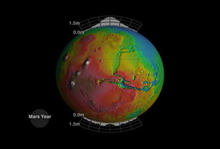
Seasonal Variations of Snow Depth on Mars
Animation showing the seasonal deposition of CO2 as measured by the Mars Orbiter Laser Altimeter on the Mars Global Surveyor spacecraft. The amplitude of the elevation change signal is greatly exaggerated for illustrative purposes.
(Credit: MOLA Science Team and G. Shirah, NASA/GSFC Scientific Visualization Studio)
Figures from the Science* Paper
* Smith, D.E., M.T. Zuber, M.T., and G.A. Neumann, Seasonal variations of snow depth on Mars, Science, 294, 2141-2146, 2001.
Download a PDF version of the paper.
Read the NASA Headquarters press release.
Read the NASA GSFC/MIT press release.
GSFC Top Story December 6.
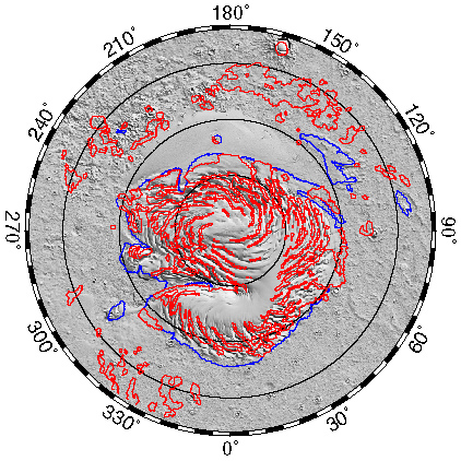
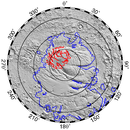
Figure 1. Shaded relief maps of (A) north and (B) south polar topography of Mars. The projection is polar stereographic from latitude 72° to the poles. The red contours in each hemisphere represent the approximate extent of the residual ice caps (denoted by high albedo), while the blue contours trace regions of elevated polar layered terrains. (Credit: MGS MOLA and RS Science Teams)
Figure 2. Latitudinal profiles of elevation change over the course of the MGS mapping mission and martian seasons (solar longitude Ls) in the (A) north polar, (B) north mid-latitude, (C) south polar, and (D) south mid-latitude regions. Shown in (A) and (B) is the time of regional dust storms that warmed the atmosphere and caused off-season sublimation in the northern hemisphere. Elevation changes in the northern hemisphere are with respect to latitude 60° N and in the southern hemisphere with respect to 60° S.
(Credit: MGS RS and MOLA Science Teams)
Figure 3. Minimum and maximum elevation changes in the northern (blue) and southern (red) hemispheres as a function of latitude over the course of a martian year. The black arrow shows the southernmost extent of the north polar residual ice cap. Note that on the north polar cap the accumulation is greater than expected from the quasi-linear latitudinal trend that characterizes both hemispheres equatorward of 80°. (Credit: MGS MOLA and RS Science Teams)
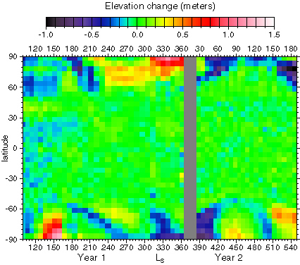
Figure 4. Temporal distribution of elevation change on Mars from MOLA crossovers. Crossover residuals are averaged over 15-day intervals, plotted as a function of latitude and Ls. Cooler hues denote regions with lower-than-average topography, while warmer hues denote higher-than-average topography. The grey zone corresponds to a data gap around Mars solar conjunction. A discontinuity at Ls=163° in year 1 reflects a one-time change in threshold on MOLA's first trigger channel. (Credit: MGS MOLA and RS Science Teams)
Figure 5. Condensed CO2 mass inferred from seasonal elevation changes of MOLA topography assuming a density of condensed material of 1000 kg m-3. MGS mapping began at Ls=103° and results are shown for more than one martian year to demonstrate the repeatability of the cycle of mass exchange. The peaks in surface mass are observed in late winter in each hemisphere. (Credit: MGS MOLA and RS Science Teams)

Figure 6. (A) Observed seasonal variation of the planetary flattening (C2,0 gravity field term), along with a fit (black line) consisting of annual, semi-annual and tri-annual terms. (B) Semi-annual component of the C2,0 gravity variation, the value predicted from MOLA elevation changes, and the C2,0 from a general circulation model (GCM) simulation of a typical seasonal cycle of CO2 exchange. (Credit: MGS MOLA and RS Science Teams)
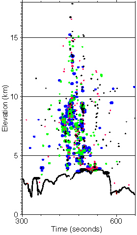
Supplementary Figure 1. Altimetric profile of Mars taken on MGS orbit 10220 1999 MAR 27 00:12 UTC over the south polar cap, 87° S, at Ls= 115.5°. The profile shows reflections from terrain (black plus signs) and atmosphere (colored ellipses). Atmospheric returns, which represent condensation of CO2 snow over the martian south polar cap, are colored black, red, green, and blue, to represent triggers by MOLA matched filter channels 1-4. Ellipse size is scaled to the strength of the returned signal. Atmospheric returns were detected at altitudes as high as 18 km during polar night. Vertical exaggeration 100:1. (Credit MGS MOLA and RS Science Teams)
Supplementary Fig. 2. Examples of annuli of topography (red) and median surfaces (blue) at latitudes 85° N, 82° N, 75° N and 60° N. Note the significant differences in the topography of different annuli that nonetheless result in similar patterns of seasonal elevation change. (Credit: MGS MOLA and RS Science Teams)
Supplementary Figure 3. Residuals representing the difference between topography and the median surface for the annuli in Web Fig. 2. Large residuals are a consequence of local topography and were smoothed. (Credit MGS MOLA and RS Science Teams)
Supplementary Figure 4. Time of year of zonal distribution of maximum CO2 accumulation measured by MOLA compared to that predicted by a general circulation model (GCM) simulation. At high latitudes the observed elevation change and GCM are in reasonable agreement, with the maximum at most latitudes occurring slightly earlier than predicted by the GCM. At lower latitudes the phase of the seasonal signal is not as well constrained, but there is evidence for transient CO2 accumulation at these latitudes during the summer. (Credit MGS MOLA and RS Science Teams)
Supplementary Figure 5. Condensed mass as a function of latitude in northern and southern hemispheres. The black arrow corresponds to the edge of the north polar residual ice cap. Note the greater accumulated mass on the north polar cap compared to that at corresponding southern latitudes. The dashed lines represent an extrapolation to correct for deposited mass that we may not have measured equatorward of latitude 60°. (Credit MGS MOLA and RS Science Teams)
Back to MOLA home
page
Direct inquiries to: zuber@tharsis.gsfc.nasa.gov